An overview of Taylor series

A fourier expansion is a way for us to approximate a function. If you've taken calculus before, you may have heard of a similar concept, Taylor series. With Taylor series, we can approximate any function as a sum of polynomials. For example, we can write \( \sin x \) as

\[ \sin x = x - \frac{x^3}{3!} + \frac{x^5}{5!} - \frac{x^7}{7!} + \cdots \]

If we were to graph this, we see that as more terms are added, our approximation becomes more and more accurate. Here's a small demonstration.

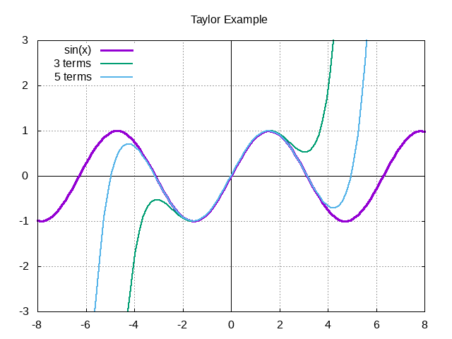
In the graph below, I tried demonstrating how the Taylor series can "home in" on a function. Since we can't add part of a term in a Taylor series, I tried to demonstrate this effect by multiplying the term by a value. For example, when you see 1.1 terms, that means the first term + 0.1 * the second term. For \( \sin x \), that's \( x - 0.1 * \frac{x^3}{3!} \)

Now, Taylor series can be useful, but they have significant limitations. First, we see that the Taylor series does a poor job modeling periodic functions. Even though \( \sin x \) repeats, our Taylor series does not. At large \(x\) values, this Taylor series is completely wrong!

Second, a Taylor series relies on the function being continuous (no holes or jumps). In addition to the function being continous, its derivatives must be as well. Let's consider the following graph.

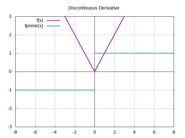
Even though \( f(x) \) is continuous, its derivative \( f'(x) \) is not. As such, a Taylor series cannot be used to approximate this function. This issue would come up even if \( f''''''''''(x) \) was discontinuous. (Keep in mind that discontinuous is not the same thing as 0! We can model \( f(x) = x \) as a Taylor series, as its higher order derivatives are continuous. They just also happen to be 0. Also, \( f(x) = x \) is its own Taylor series.)

So, to summarize, Taylor series have the following issues

1. They do not model periodic functions well

2. They require the function and all of its derivatives to be continuous

Fortunately, the Fourier series provides answers to both of these problems! (At least for most functions. Some functions, like a function that is discontinuous everywhere, exist solely for the purpose of making us sad.)

What we're all here for, Fourier series

I'll be sticking to the basics of Fourier series for now. Let's assume we have a periodic function \( f(x) \) that has a period of \( T \). I am going to introduce the symbol \( l \) where \( l = \frac{T}{2} \) While this isn't the only option, we can write the Fourier series as

\[ f(x) = \sum_{n=0}^{\infty} a_n \cos(\frac{n \pi x}{l}) + b_n \sin(\frac{n \pi x }{l} ) \]

In this case, we can find \( a_n \) and \( b_n \) with the formulas

\[ a_n = \frac{1}{l} \int_{0}^{2l} f(x) \cos(\frac{n \pi x }{l}) dx \]

\[ b_n = \frac{1}{l} \int_{0}^{2l} f(x) \sin(\frac{n \pi x }{l}) dx \]

I won't go into detail as to where these formulas come from. (That is left as an exercise for the reader. Hah!) However, I will point out that we can adjust the limits of integration to any values we want, just as long as the difference between the upper and lower limits equals our period.

There is one special case that we need to discuss. When \( n = 0 \), we need a new formula for \( a_0 \). This formula will look like

\[ a_0 = \frac{1}{2l} \int_{0}^{2l} f(x) dx \]

Fortunately there is no special case for \( b_0 \). This occurs due to the fact that \( a_0 \) is a constant term ( \( \cos 0 = 1 \) as opposed to periodic.

That is all the theory that we need to calculate the Fourier series! As long as we can find a library that can perform integration for us, we should be able to calculate the Fourier series for any periodic function.

Using GSL to calculate an integral

Explanation of gsl_integration_qng()

Because of inscrutible magic mumbo jumbo, I decided to use C for calculating the Fourier expansion. In order to do that, I needed to pick out a library that could perform the integration for me. I settled on GSL or the GNU Scientific Library. There are many, many, MANY functions available in this library, but luckily I only need to worry about integration.

Before going too far into Fourier stuff, I'm going to do a simple sanity check so I can make sure I'm calculating integrals correctly. I want to calculate the following integral.

\[ \int_{0}^{8} x dx \]

To do this using GSL, I can use the gsl_integration_qng() function. This function has the following signature.

  int gsl_integration_qng(const gsl_function * f,
              double a, double b,
              double epsabs, double epsrel,
              double * result, double * abserr,
              size_t * neval)

f is a pointer to a structure that contains a function pointer. For those who don't speak nerd, this is how gsl_integration_qng() knows what function to integrate. It's our f(x). (Mostly. The reason for making it a structure is because the structure also contains a void * or void pointer. This void pointer can be used to pass parameters to the function. This could be used to let us change the slope of the function without having to modify the function itself.

a and b are the lower and upper limits of integration. That's fairly straightforward.

epsabs and epsrel help gsl_integration_qng() decide when to stop integrating. It's not possible to integrate the function to an exact value with GSL. Instead, it tries to zero in on a specific value or best guess as to what the answer is. epsabs is the absolute error that we want. If epsabs = 0.1, we don't know what the answer is, but we know we are no more than 0.1 away from it. epsrel is similar, but percentage based instead of absolute. (e.g. epsrel = 0.01 means our answer is within 1% of the actual value.)

result and abserr are used by the function to store the result and estimated absolute error, respectively. The number of iterations it took to calculate the result is stored in neval.

It is possible for the integration to fail. This might happen if we set the error tolerances too tight. Since the function we're integrating is so simple, I don't think that's a likely concern.

gsl_integration_qng() in use

To compile this program, you will need to tell the compiler what external libraries to use. You can do with with the -lgsl compile flag, e.g. gcc main.c -lgsl. Because GSL depends on another library, CBLAS, you will also need the -lcblas flag. If CBLAS isn't available, you can use a version of CBLAS provided by GSL with -lgslcblas. (Don't forget to install GSL!) Since I'm using some math function, I'm also going to include the math library with -lm.

In the end, our command will look like gcc main.c -lgsl -lcblas -lm, which will compile =main.c= and create an output file =a.out=. (Actually I'm using =org-babel= so I don't have to deal with this, but I'm assuming most readers here are not.)

Alright! Time to integrate! I need to preface the gsl_integration.h header withgsl/as the headers are installed in agsl` subdirectory. (If you installed this through your systems package manager, you can probably find this file in =/usr/include/gsl/=.)

  #include <stdio.h>
  #include <gsl/gsl_integration.h>
  #include <math.h>

  /* This is where we define the function */
  double f(double x, void *params) {
    return x;
  }

  int main() {
    double result, error;
    double low = 0, high = 8;
    gsl_function F = {.function = &f};
    double err_abs = 0, err_rel = 1;
    size_t num_evals;

    gsl_integration_qng(&F, low, high, err_abs, err_rel,
            &result, &error, &num_evals);
    printf("result error num_evals\n");
    printf("%f %f %zu\n", result, error, num_evals);
  }

#+RESULTS:

| result | error | num_evals |
|   32.0 |   0.0 |        21 |

There we go! GSL was able to successfully integrate \( \int_{0}^{8} x dx \).

In the next part, we'll start using GSL to calculate the Fourier series of a discontinuous, periodic function. We'll see if we can naively get away with using the simple gsl_integration_qng() function, or if we need to find a more complicated, but more powerful, alternative.